
Eigen-vesting II. Optimize Your Portfolio With Optimization
Table of Contents
In the last post, we talked about using eigenportfolios for investing. To continue the series, we are going to present more of Markowitz Portfolio Theory. In particular, we will demonstrate how optimization yields the Minimum Variance Portfolio.
Minimum Variance Portfolio
We are going to use the notation from the last post. For a universe of \(N\) stocks, let \(\Sigma\) be the covariance matrix and \(w\) the corresponding allocation weight for each stock arranged as a vector. Then, the Minimum Variance Portfolio is the solution to the following problem: \begin{equation} \min_{w} w^T \Sigma w \end{equation} subject to \begin{equation} w^T \mathbb{1} = 1\end{equation}
where \(\mathbb{1}\) is a vector of 1’s. This problem has the unique solution \begin{equation} w = \frac{ \Sigma^{-1}\mathbb{1} }{ (\Sigma^{-1}\mathbb{1})^T \mathbb{1} }. \end{equation}
This solution depends on the covariance matrix, which is of course estimated from data. Even if we had access to the true covariance matrix, the covariance matrix changes over time. This means that your estimate of the true Minimum Variance Portfolio will change as well, and you will have to alter your investments occasionally with this technique. Occasionally, you should rebalance your portfolio, and at that time you could update the covariance matrix.
Proof
If you define the function \begin{equation} \mathcal{L}(w,\lambda) := w^T\Sigma w + \lambda (w^T \mathbb{1} - 1), \end{equation} then since \(\Sigma\) is symmetric, the quadratic part is positive definite and a unique minimizer exists and occurs at \((w,\lambda)\) such that \(\nabla \mathcal{L}(w,\lambda) = (0,\dots,0)^T.\) Solving this equation gives two equations that are satisfied: from the \(\lambda\) component of the gradient we recovery the constraint \(w^T \mathbb{1} = 1\). From the top \(N\) components associated with \(w\), we have the equation (after some algebra) \begin{equation} \Sigma w = -\lambda \mathbb{1}. \end{equation} If \(\Sigma\) is invertible, then the unique solution is \begin{equation} w = -\lambda \Sigma^{-1}\mathbb{1} = \frac{ -\lambda \Sigma^{-1}\mathbb{1} }{1}. \end{equation} By substituting the constraint in for the denominator, we eliminate \(-\lambda\) to have the solution: \begin{equation} w = \frac{ -\lambda \Sigma^{-1}\mathbb{1} }{w^T \mathbb{1} } = \frac{ -\lambda \Sigma^{-1}\mathbb{1} }{ (-\lambda \Sigma^{-1}\mathbb{1})^T \mathbb{1} } = \frac{ \Sigma^{-1}\mathbb{1} }{ (\Sigma^{-1}\mathbb{1})^T \mathbb{1} }. \end{equation}
Example
We’re going to use the code from the last post and expand upon it with our new analytical tool. First, we get the data as we did before:
1
2
3
4
5
6
7
8
9
10
11
12
13
14
    import pandas as pd
    import datetime as dt
    from pandas.io.data import DataReader

    start, end = dt.datetime(2012, 1, 1), dt.datetime(2013, 12, 31)
    tickers = ['AAPL', 'YHOO','GOOG', 'MSFT','ALTR','WDC','KLAC']
    prices = pd.DataFrame()
    for ticker in tickers:
        prices[ticker] = DataReader(ticker,'yahoo', start, end).loc[:,'Close'] #S&P 500
    returns = prices.pct_change()
    returns = returns.iloc[1:, :] # Remove first row of NA's
    training_period = 30
    in_sample = returns.iloc[:(returns.shape[0]-training_period), :].copy()
    tickers = returns.columns.copy() # Save the tickers
Now, we’re going to calculate the inverse of the covariance matrix using a pseudo-inverse (incase it is ill-conditioned or singular) and then construct the minimum variance strategy weights.
1
2
3
4
5
6
7
8
9
10
11
12
import numpy as np
covariance_matrix = in_sample.cov().values
inv_cov_mat = np.linalg.pinv(covariance_matrix) # Use pseudo-inverse incase matrix is singular / ill-conditioned
# Construct minimum variance weights
ones = np.ones(len(inv_cov_mat))
inv_dot_ones = np.dot(inv_cov_mat, ones)
min_var_weights = inv_dot_ones/ np.dot( inv_dot_ones , ones)
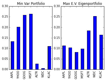
min_var_portfolio = pd.DataFrame(data= min_var_weights, columns = ['Investment Weight'], index = tickers)
min_var_portfolio
| Investment Weight | |
|---|---|
| AAPL | 0.133215 |
| YHOO | 0.196214 |
| GOOG | 0.260885 |
| MSFT | 0.261103 |
| ALTR | 0.023642 |
| WDC | 0.006199 |
| KLAC | 0.118743 |
We will also compare it to the largest eigenvalue’s eigenportfolio:
1
2
3
4
5
6
7
8
9
10
11
12
13
14
15
16
    # Largest eigenvalue eigenportfolio
    D, S = np.linalg.eigh(covariance_matrix)
    eigenportfolio_1 = S[:,-1] / np.sum(S[:,-1]) # Normalize to sum to 1
    eigenportfolio_largest = pd.DataFrame(data= eigenportfolio_1, columns = ['Investment Weight'], index = tickers)

    # Plot
    %matplotlib inline
    import matplotlib.pyplot as plt
    f = plt.figure()
    ax = plt.subplot(121)
    min_var_portfolio.plot(kind='bar', ax=ax, legend=False)
    plt.title("Min Var Portfolio")
    ax = plt.subplot(122)
    eigenportfolio_largest.plot(kind='bar', ax=ax, legend=False)
    plt.title("Max E.V. Eigenportfolio")
    print(min_var_portfolio)
      Investment Weight
AAPL           0.133215
YHOO           0.196214
GOOG           0.260885
MSFT           0.261103
ALTR           0.023642
WDC            0.006199
KLAC           0.118743
Now let’s test the algorithm on returns data and compare it to the eigenprofile related to the largest eigenvalue.
1
2
3
4
5
6
7
8
9
10
11
12
13
14
15
16
17
18
19
20
21
    def get_cumulative_returns_over_time(sample, weights):
        return (((1+sample).cumprod(axis=0))-1).dot(weights)

    in_sample_ind = np.arange(0, (returns.shape[0]-training_period+1))
    out_sample_ind = np.arange((returns.shape[0]-training_period+1), returns.shape[0])

    cumulative_returns = get_cumulative_returns_over_time(returns, min_var_portfolio).values
    cumulative_returns_largest = get_cumulative_returns_over_time(returns, eigenportfolio_largest).values


    f = plt.figure(figsize=(10,4))

    ax = plt.subplot(121)
    ax.plot(cumulative_returns[in_sample_ind], 'black')
    ax.plot(out_sample_ind,cumulative_returns[out_sample_ind], 'r')
    plt.title("Minimum Variance Portfolio")

    ax = plt.subplot(122)
    ax.plot(cumulative_returns_largest[in_sample_ind], 'black')
    ax.plot(out_sample_ind,cumulative_returns_largest[out_sample_ind], 'r')
    plt.title("Eigenportfolio")
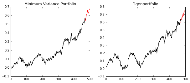
The minimum variance portfolio did not beat the eigenportfolio (with the most variance), but it had less variance! Usually, this type of portfolio could be blended with other strategies to try to guarantee some returns in bad times. If we didn’t trust our math, we could calculate this variance like so for verification:
1
2
3
4
5
6
    # Variance = w^T Sigma w
    largest_var = np.dot(eigenportfolio_1, np.dot(covariance_matrix, eigenportfolio_1))
    min_var = np.dot(min_var_weights, np.dot(covariance_matrix, min_var_weights))

    print('The eigenportfolio has a variance of %f.\nThe minimum variance portfolio has a variance of %f'
          % (largest_var,min_var))
The eigenportfolio has a standard deviation of 0.000139.
The minimum variance portfolio has a standard deviation of 0.000092
Additional Modeling Constraints
You can extend this problem by adding more constraints or terms to the function we with to optimize.
“Efficiency” Portfolios
Let \(\mu\) be a vector of expected (linear) returns for each stock. Then you can calculate the minimum variance portfolio according to a given return \(\gamma\) for a period \begin{equation} \min_{w} w^T \Sigma w \end{equation} subject to \begin{equation} w^T \mathbb{1} = 1\end{equation} \begin{equation} w^T \mu = \gamma. \end{equation} Notice, this approach gives you the minimum variance for a set return over a period… hence, “efficiency”. This formulation also has an exact solution that can be solved via Lagrange multipliers.
No Short Sales
Adding the constraints \(w_i \geq 0\) for all stocks \(i\) to any portfolio optimization problem will give us a solution with no short sales. This already would make life much easier for a basic backtesting algorithm, and for the common investor to implement as an investing strategy. However, this problem would typically be solved with a quadratic programming solver (not analytically like we have done thus far).