
Learning RecSys through Papers- Implementing a Candidate Generation Model
Table of Contents
Sometimes I’m asked how to start learning about recommender systems, and there’s a few go-to papers I always mention; however, without a proper map, it could be alittle difficult for the uninitiated. So, to try to make a gentle introduction, I will walk through an implementation of the candidate generation model based on Deep Neural Networks for YouTube, which I will sometimes refer to as the “Deep Nets” paper. This paper (and its talk) is jam-packed with all sorts of interesting practical recommendation system knowledge and is the perfect starting place for people hoping to understand large-scale recommendation systems. I will implement the key components of the candidate generation model and train the model on the MovieLens dataset in PyTorch, a typical benchmark dataset in the RecSys space. There will also be a few modern flourishes and comments on new developments as applicable. I’ll conclude with outlining a natural extension to this approach to predict multiple outcomes.
Candidate Generation
A recommendation system is like a funnel that starts from the largest pool of content avaialble to a user and filters until we get the right set of items to show to a user. From the paper, they have the following graphic that illustrates the process well:
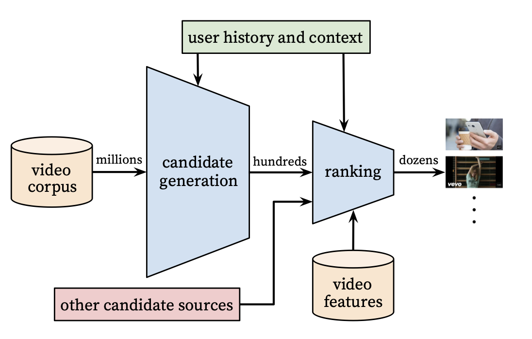
Our goal is to find items in the (possible) billions of possible items to present to the user to improve upon given business metrics. We do this by modeling the problem as “predicting what the user will watch” with watched items being positive examples and unwatched items being negatives. In the next sections, we will detail modeling decisions for various components and data preparation.
Modeling
For the uninitiated, recommendation systems are basically a big vector search if you squint at it. We represent users and items as vectors and then using approximate lookup techniques we can scale the search to very large item sets. The first step in the pipeline is the candidate generation where a user vector is generated and used to look up candidate items via approximate nearest neighbor techniques (e.g., Hierarchical Navigatable Small Worlds). When using matrix factorization methods, each user has a vector that is learned during training. In neural methods for recommenders, typically features like watch history among others are passed into neural nets to generate user embeddings.
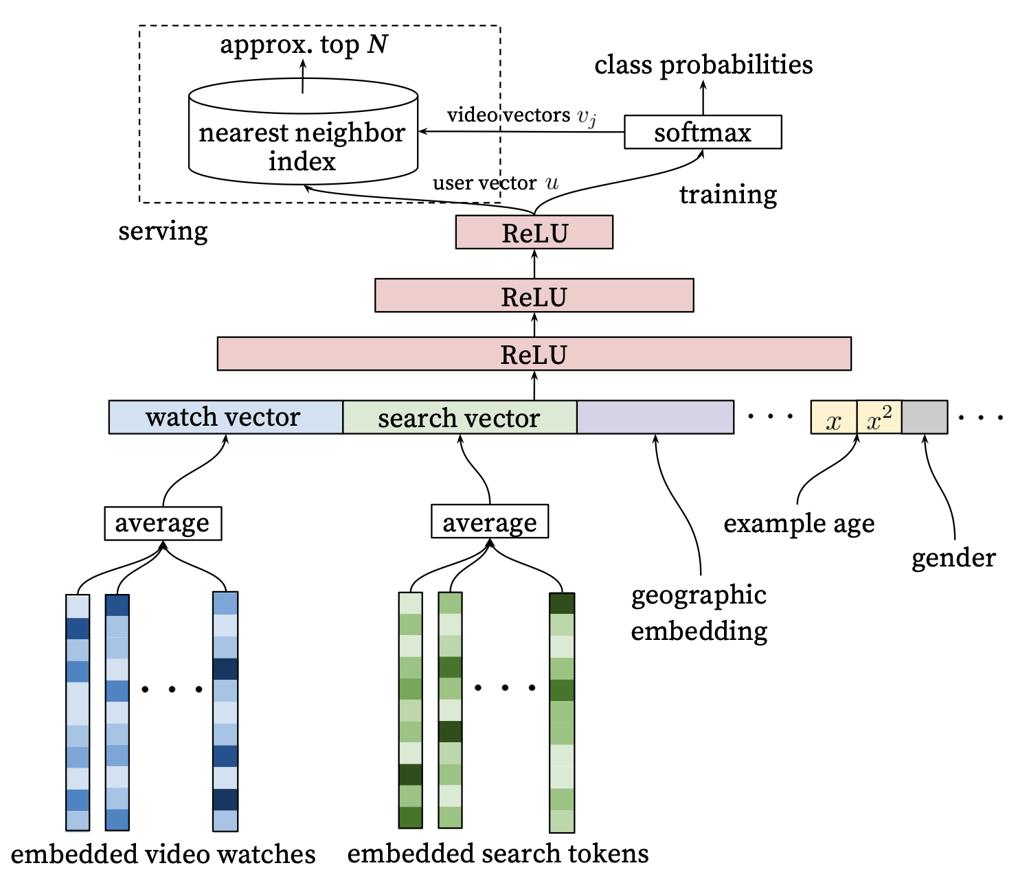
In the YouTube Deep Nets paper, various user level features are fed into a feedforward network to generate a user vector which is then passed into a dense layer leading to a big softmax, where every item corresponds to an index in the softmax’s output.
For training, the dense layer for the softmax would become prohibitivelty large, and so variations on a sampled softmax are typically used. Indeed, even the input embedding layers have a similar issues, and more modern techniques would use things like Hash Embeddings and other tricks to reduce the size of the embedding table (e.g., see TikTok describe its collisionless embedding table).
In my implementation, I will use a simplified shared hash embeddings to represent both the watched item IDs and the softmax output, combined with sampled softmax. Shared embeddings is a common technique used in such systems and can improve generalization, as stated in the YouTube Deep Nets paper in Section 4.1:
Sharing embeddings is important for improving generalization, speeding up training and reducing memory requirements. The overwhelming majority of model parameters are in these high-cardinality embedding spaces - for example, one million IDs embedded in a 32 dimensional space have 7 times more parameters than fully connected layers 2048 units wide.
A user will be represented by a list of past watched item IDs. You will notice in my implementation I allow variable length watch histories up to length max_pad=30. I do this by looping over the inputs, applying the embedding layer, and then averaging the inputs. Treating items as a “bag of words” is a common approach in early recommender systems, especially before the onset of Transformers and efficient RNNs. The approach is still extremely effective when combined with side features, such as in the Deep Nets Youtube paper and the Wide and Deep paper.
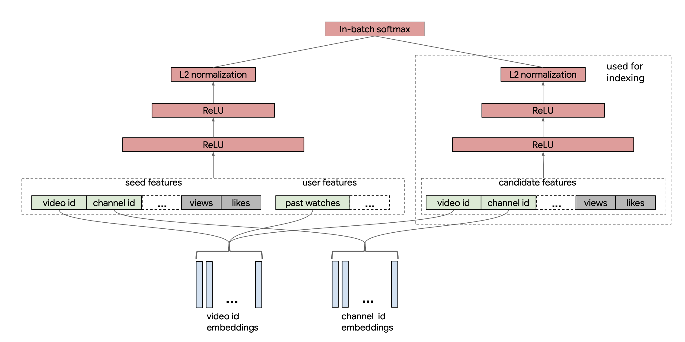
My network architecture is closer to a two-tower architecture, which became more common in later papers such as this paper from YouTube in 2019. In the paper, they actually use in-batch items as their negatives but need to perform a correction to account for popular items showing up more often in their loss. I take this idea of the two-tower achitecture with shared embeddings and I remove the candidate tower and simply pass through the item embeddings to dot with each input item. The main difference is I do not use in-batch negatives but instead will sample negatives at random per example. You can see the two-tower architecture from the paper below and imagine that we pass the video embeddings directly through the right-hand side item tower to lead to the softmax term:
import torch
import torch.nn as nn
import torch.nn.functional as F
import hashlib
import pandas as pd
import numpy as np

EMBED_TABLE_SIZE = 1000
hash_f = lambda x: int(hashlib.md5(x.encode('utf-8')).hexdigest(),16) % EMBED_TABLE_SIZE
mps_device = torch.device("mps")
max_pad=30
class DeepNetRecommender(nn.Module):
    def __init__(self, n_embed=3, table_size=EMBED_TABLE_SIZE, embed_dim=64):
        super(DeepNetRecommender, self).__init__()
        # MUST DEFINE ALL LAYERS IN THE BODY OR PYTORCH DOESNT NOTICE THEM
        self.embed1 = nn.Embedding(table_size, embed_dim)
        self.embed2 = nn.Embedding(table_size, embed_dim)
        self.embed3 = nn.Embedding(table_size, embed_dim)

        # need to set seed for it to be the same every load
        np.random.seed(182)
        self.embeds = [(getattr(self,'embed'+str(k)),np.random.choice(100000)) for k in range(1,1+n_embed)] # (layer, salt)

        self.model = nn.Sequential(nn.Linear(64,64), nn.ReLU(), nn.Linear(64,64), nn.ReLU(), nn.Linear(64,64))

    def embed(self, x, max_pad):
        o = None
        for embedder, salt in self.embeds:
            items = [hash_f(str(salt) + '_' + str(k)) for k in x][:max_pad]
            hashed_items = torch.IntTensor(items).to(mps_device)
            embedded = embedder(hashed_items)
            if o is None:
                o = embedded
            else:
                o += embedded
        return o

    def embed_stack(self, x):
        return torch.stack([self.embed(k, max_pad=len(k)) for k in x],0)

    def _embed_transform(self, y, max_pad):
        # embeds variable length inputs and translate them to the same size, [1,64] via averaging
        x = self.embed(y, max_pad)
        return torch.sum(x,0) / x.shape[0]

    def embed_and_avg(self, data, max_pad):
        stacked = torch.stack([self._embed_transform(x, max_pad) for x in data],0)
        return stacked.unsqueeze(1)

    def forward(self, x):
        # Pad, stack and embed vectors
        inps = x['history']
        to_rank = x['to_rank']

        lhs = self.embed_and_avg(inps, max_pad)
        lhs = self.model(lhs)

        rhs = self.embed_stack(to_rank)

        output = torch.bmm(lhs, rhs.T.permute(-1,0,1))
        return output.squeeze(1)
As I mentioned before, we are using a sampled softmax approach. If your softmax output dimension is one-to-one with your item catalog, you can use functions build into PyTorch to sample indices. To create the sampled softmax, I reuse the simplified hash embedding by dotting the item vector with the user embedding, and therefore, I have to explicitly pass in valid item IDs to ensure I am learning embeddings on the items I care about. In practice, it’s more likely to see the output item vectors independent of the inputs for these types of models as it allows for easier sampling without knowing the identifiers of the items you are sampling.
model = DeepNetRecommender().to(mps_device)

with torch.no_grad():
    print(
        model({'history': [[1,182,1930]], 'to_rank': [[1,8,24,1234,53435,1000000]]}).cpu().detach()
    )
tensor([[ 3.3182, -0.1267, -0.1815, -0.1327, -0.0200, -0.4532]])
Data Processing
There are two approaches to modeling the data presented in the paper. I will focus on the one I find works best in practice– the “predicting the next/future watch”:
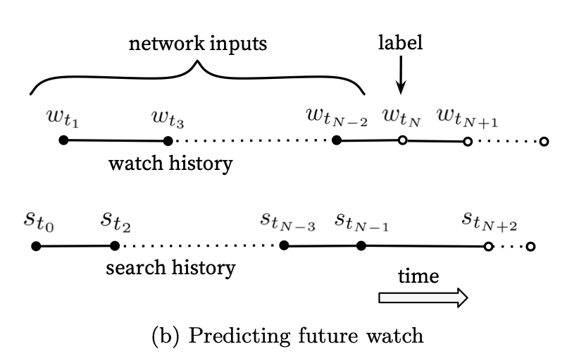
Here, you take all the information leading up to a watch as your inputs and predict the item that will be watched. Notice, this approach only requires positive samples as the softmax will imply the other examples are the negatives. We will use the MovieLens dataset, sorted by time, and do a groupby on each user to get a big ordered list for each user. Then in our training loop, we will sample an index as our watch item and generate the appropriate history window (considering our max_pad parameter). We will do all this in a custom DataLoader class. Here I will also sample item IDs in the data loader and output them as the label and pass that into the model during training to score each label ID. For the sampled softmax, we will take 1000 items in total to calculate the loss for each training instance.
d = pd.read_csv('data/ratings.csv')
n_movies = d.movieId.nunique()
all_movies = d.movieId.unique().tolist()
n_movies
83239
d['click'] = d['rating'] >= 3 # Ratings bigger than 3 we consider a click/watch
dd = d[d['click'] > 0].groupby('userId', as_index=False).movieId.apply(list) # assumes final list is in order
dd.set_index('userId',inplace=True)
dd=dd[dd.movieId.apply(len) > max_pad+2] # minimum number of movies per user
from torch.utils.data import Dataset
class MovieLensDataset(Dataset):
    def __init__(self, user_level_data, random_negatives=999):
        self.d = user_level_data
        self.rn = random_negatives

    def __len__(self):
        return len(self.d)

    def __getitem__(self, idx):
        user_movies = dd.iloc[idx]['movieId']
        label_idx = np.random.choice(range(1,len(user_movies)))
        history = user_movies[label_idx-max_pad:label_idx]
        label_movie_id = user_movies[label_idx]
        # sample real movie ids so we get reasonable embedding lookups.. as it's not a true softmax
        to_rank = [label_movie_id] + np.random.choice(all_movies, self.rn).tolist()
        start_idx = label_idx-max_pad if label_idx-max_pad > 0 else 0
        movies = user_movies[start_idx:label_idx]
        if len(movies) == 0:
            print('FAIL', label_idx, start_idx, t_rank)
        return movies, to_rank
Training
This section is mostly boilerplate PyTorch code.
from torch.utils.tensorboard import SummaryWriter

writer = SummaryWriter('runs/experiment_1')

loss_fn = torch.nn.CrossEntropyLoss() # not equiv to Keras CCE https://discuss.pytorch.org/t/categorical-cross-entropy-loss-function-equivalent-in-pytorch/85165/11
optimizer = torch.optim.Adam(model.parameters(), lr=0.01)
dd['train'] = np.random.uniform(0,1, len(dd)) < .9

dataset=MovieLensDataset(dd[dd['train']])
val_dataset=MovieLensDataset(dd[~dd['train']])

def my_collate(batch):
    data = [item[0] for item in batch]
    target = [item[1] for item in batch]
    target = target
    return [data, target]

trainloader = torch.utils.data.DataLoader(dataset, batch_size=256, drop_last=True,
                                        shuffle=True, collate_fn = my_collate)
testloader = torch.utils.data.DataLoader(val_dataset, batch_size=256, drop_last=True,
                                        shuffle=True, collate_fn = my_collate)
def train_one_epoch(epoch_index, tb_writer):
    running_loss = 0.
    last_loss = 0.

    for i, data in enumerate(trainloader):
        inputs, labels = data
        optimizer.zero_grad()

        # Make predictions for this batch

        outputs = model({'history': inputs, 'to_rank':labels})

        # Compute the loss and its gradients
        default_label = torch.zeros((outputs.shape[0]), dtype=torch.long).to(mps_device)
        loss = loss_fn(outputs, default_label)
        loss.backward()

        # Adjust learning weights
        optimizer.step()

        # Gather data and report
        l = loss.item()
        running_loss += l
        if i % 100 == 99:
            last_loss = running_loss / 100 # loss per batch
            print('  batch {} loss: {}'.format(i + 1, last_loss))
            tb_x = epoch_index * len(trainloader) + i + 1
            tb_writer.add_scalar('Loss/train', last_loss, tb_x)
            running_loss = 0.

    return last_loss
fixed_validation_set = [vdata for vdata in testloader]

for epoch_number in range(1):

    model.train()
    avg_loss = train_one_epoch(1, writer)

    running_vloss = 0.0
    model.eval()

    with torch.no_grad():
        for i, vdata in enumerate(fixed_validation_set):
            vinputs, vlabels = vdata
            voutputs = model({'history': vinputs, 'to_rank':vlabels})
            default_label = torch.zeros((voutputs.shape[0]), dtype=torch.long).to(mps_device)
            vloss = loss_fn(voutputs, default_label)
            running_vloss += vloss

    avg_vloss = running_vloss / (i + 1)
    print('LOSS train {} valid {}'.format(avg_loss, avg_vloss))

    writer.add_scalars('Training vs. Validation Loss',
                    { 'Training' : avg_loss, 'Validation' : avg_vloss },
                    epoch_number + 1)
    writer.flush()

    torch.save(model, 'model.pt' +'_' +'_'.join([str(k[1]) for k in model.embeds]) +'.pt' ) # save model with hashes
  batch 100 loss: 6.049025082588196
  batch 200 loss: 4.822506718635559
  batch 300 loss: 4.121425771713257
  batch 400 loss: 3.6819806337356566
  batch 500 loss: 3.45309770822525
LOSS train 3.45309770822525 valid 3.265143871307373
Example Prediction
movies = pd.read_csv('data/movies.csv')
movies.set_index('movieId',inplace=True)
def map_movies_list(x):
    return [movies.loc[k,'title'] for k in x]
all_movies_scored = model({'history': [dd.iloc[0].movieId[:max_pad]], 'to_rank': [list(movies.index)]})
print('User Movies','\n', map_movies_list(dd.iloc[0].movieId[:max_pad]))
User Movies
 ['Toy Story (1995)', 'Braveheart (1995)', 'Casper (1995)', 'Star Wars: Episode IV - A New Hope (1977)', 'Forrest Gump (1994)', 'When a Man Loves a Woman (1994)', 'Pinocchio (1940)', 'Die Hard (1988)', 'Ghost and the Darkness, The (1996)', 'Shall We Dance (1937)', 'Star Wars: Episode V - The Empire Strikes Back (1980)', 'Aliens (1986)', 'Star Wars: Episode VI - Return of the Jedi (1983)', 'Alien (1979)', 'Indiana Jones and the Last Crusade (1989)', 'Star Trek IV: The Voyage Home (1986)', 'Sneakers (1992)', 'Shall We Dance? (Shall We Dansu?) (1996)', 'X-Files: Fight the Future, The (1998)', 'Out of Africa (1985)', 'Last Emperor, The (1987)', 'Saving Private Ryan (1998)', '101 Dalmatians (One Hundred and One Dalmatians) (1961)', 'Lord of the Rings, The (1978)', 'Elizabeth (1998)', 'Notting Hill (1999)', 'Sixth Sense, The (1999)', 'Christmas Story, A (1983)', "Boys Don't Cry (1999)", 'American Graffiti (1973)']
print('Predicted Top 20 Movies', '\n', movies.title.values[np.argsort(all_movies_scored.cpu().detach().numpy())[0][::-1]][:20])
Predicted Top 20 Movies
 ['Gladiator (2000)' 'Green Mile, The (1999)' 'American Pie (1999)'
 'Fight Club (1999)' 'Memento (2000)' 'Being John Malkovich (1999)'
 'Toy Story 2 (1999)'
 'Lord of the Rings: The Fellowship of the Ring, The (2001)'
 'Matrix, The (1999)' 'Princess Mononoke (Mononoke-hime) (1997)'
 'X-Men (2000)' 'American Beauty (1999)' 'Shrek (2001)'
 'Requiem for a Dream (2000)' 'Cast Away (2000)'
 'Ghostbusters (a.k.a. Ghost Busters) (1984)'
 'Who Framed Roger Rabbit? (1988)' 'Airplane! (1980)'
 'Crouching Tiger, Hidden Dragon (Wo hu cang long) (2000)'
 'Sixth Sense, The (1999)']
Extensions
Predicting Multiple Outcomes
In our model, we are only predicting if the user will watch an item or not. It may be that you want to predict various outcomes, like a click, a save, a buy, etc. One approach is modeling outcomes as prediction tasks demonstrated by Pinterest in their ItemSage paper. Here, they extend the basic model by adding an input term for the outcome they are predicting and embed that for each example. Then, they leverage both in-batch negatives and random negatives to train their model end-to-end. The in-batch negatives help the model learn the difference between popular items where the random negatives help to push down (i.e., rank lower) long-tail irrelevant items during inference.
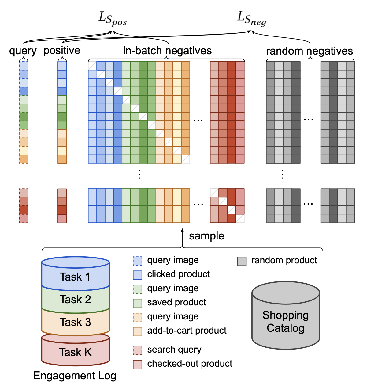
The paper discusses implementing multiple tasks in Section 3.5:
We implement multi-task learning by combining positive labels from all the different tasks into the same training batch (Figure 4). This technique is effective even when the query entities come from different modalities, the only difference being that the query embedding needs to be inferred with a different pretrained model.
Off-Policy Reinforcement Learning
Minmin Chen, the author of Top-K Off-Policy Correction for a REINFORCE Recommender System, said the model from the paper was the single biggest launch in terms of metric improvements at YouTube for that year in her talk on the topic. The recommender system is modeled as a Reinforcement Learning problem and they leverage techniques from the off-policy learning literature to correct for the “behavior policy” (i.e., their production system) which generated and biased their data. Another way to put this is that they use Inverse Propensity Scoring (IPS) in a clever way to correct for biases in their training data, allowing them to properly optimize their desired loss on their data distribution. In their approach, they learn the behavior policy as a separate task during training:
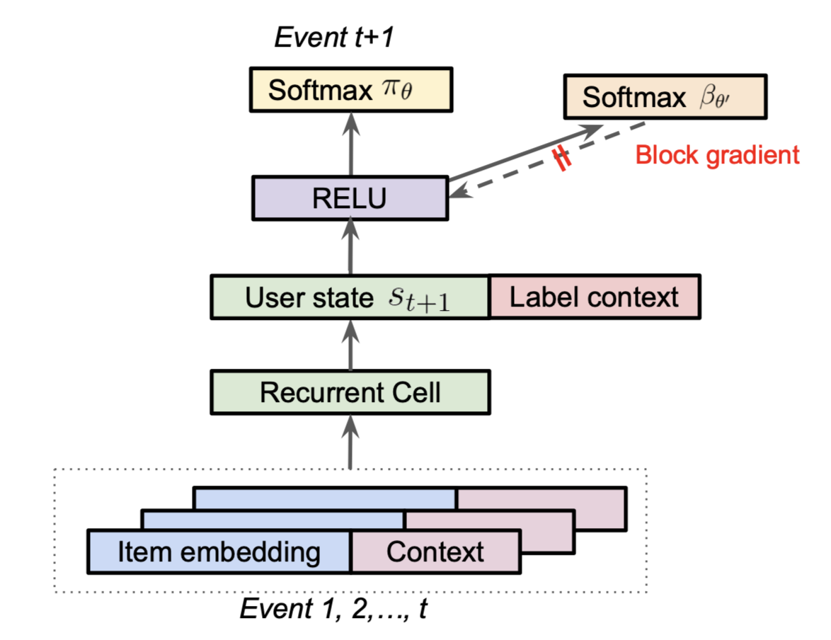
One interesting note above is to concatenate a label context to the final user state from the RNN is another way to implement a flavor of multiple tasks from the previous section.
Knowledge Graph-based Recommenders
Another avenue for improvement are different approaches to candidate generation. Knowledge graphs embed relational information among items (called entities) and can give more contextual recommendations. For example, if you watched a movie with an actor, the movie node could be connected to an actor node which is then connected to their other movies. An important paper in this space is Knowledge Graph Convolutional Networks for Recommender Systems, which embeds the knowledge graph into a vector space, allowing one to do the same retrieval techniques that we discussed above via the dot product.